Number Crunching
Digital computers work by processing streams of bits in their inputs resulting in various side effects, including producing other binary streams as output. This works because many aspects of real life have binary representations. Images, sound or printed text can encoded in binary representations and computers can be taught to operate on them such that they can serve a purpose for us. Most of the time in CP we are trying to produce numerical solutions for problems that are difficult to handle in close form or analytically, by using only paper and pencil. Therefore we have to learn how Python deals with numbers, and how computers' limitations may affect our expectations. These limitations derive from two characteristics of computer hardwares:
- the Arithmetics and Logical Unit (ALU) inside a microprocessor operates on groups of bits of fixed size. Most modern computers have 64 bit wide units.
- the memory used for storing numbers, or any other piece of information, is limited.
Because of these limitations, computers can not represent reals numbers with an infinite number of decimal places. Instead, only a countable subset of numbers get represented. This means that any computer has a largest and a smallest number can store and operate. This subset of representable numbers is very large, and more than sufficient for many CP calculations. Because of their speed and reliability we tend to attribute magic powers to the computer and trust any results that produces, and believe that the math it does is somehow perfect. However, there are situations in which limitations will affect us significantly, and even catastrophically. You may think that those are extremely rare cases, but there are stories of lost aeronautical equipment at NASA because engineers trusted the results a bit too much. It is then crucial to acknowledge and understand computer's limitations and know when and how to deal with them when necessary.
You already encountered a manifestation of this phenomenon in the example calculation of the number $\pi$ by using the Archimede's bounding procedure.
Here is another example. A simple calculation shows that $$ \frac 1{(1 + x) - 1} = \frac 1x $$
for k in range(10,20):
    x = pow(10, -k)
    y = 1/((1+x) - 1)
    print("x = ",x, "y= ", y, "\t 1/x = ", 1/x)
What is going on?
Representation of numbers
There are many representations of real numbers in a computer. We running a program we expect to produce the same result no matter of what hardware is used. That's how mathematics works. To avoid confusion and promote inter-operability a set of rules about the representation of real numbers was formulated. This is called the IEEE 754 standard.
A number in base 10 could be written like this:
        -1.234 E -02
        \____/   \_/
   significand  exponent
A floating point number is actually stored as a signed significand and signed exponent, both in base 2.
Special values for floating point numbers include -0.0, -inf, +inf, and nan.
There are technically quiet nans and signaling nans in IEEE 754, but I'm not aware of any place in Python where they are distinguished as such - both are called
nan.
If you are curious, here is an example of a binary representation of a 32-bit floating-point number.
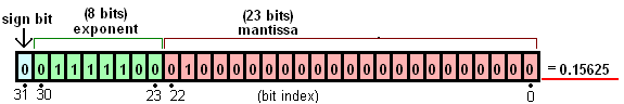
The value depicted, 0.15625, occupies 4 bytes of memory: 00111110 00100000 00000000 00000000
Common floating point types (IEEE 754 standard):
        | Significand | Exponent | Approx digits
float16 |     11      |     5    |      3-4       (half)
float32 |     24      |     8    |      7-8       (single)
float64 |     53      |     11   |     15-16      (double)
How many numbers can be represented?
print(f"16 bits: {2**16:,}\n32 bits: {2**32:,}\n64 bits: {2**64:,}")
There are also some base 2 decimal numbers, like 0.3, that can't be stored in finite digits in base 2. (Any number with a factor of 5 in the denominator). Python is smart and tries to provide a "nice" representation for you, but you can force it to show you more digits:
print(f"1/2:   {.5}   {.5:.30f}")
print(f"1/5:   {.2}   {.2:.30f}")
print(f"1/10:  {.1}   {.1:.30f}")
print(f"3/30:  {.3}   {.3:.30f}")
In Python real numbers can only be of the type double precision, which means that the precision of significand is limited to 52 bits of precision, which converts to 15 to 16 base-10 digits of precision. The trouble pops up when we try to add a very large number to a very small number resulting in a rounding error.
1.0000000000000000 + 0.0000000000000001
This is an extreme case illustrating the problem. But when starting a calculation, say with the maximum number of digits of precision, 16 for all terms and factor, the precision of the results always decreases a little bit or more, depending on the difference in magnitude and on the type of the operations involved. In the worst case, at the end of a lengthy calculation, it can happen that ALL digits are lost, and the results may be useless. Python may catch situations of overflow (numbers greater than $\approx 10^{308}$)or underflow (numbers smaller than $\approx 10^{-308}$ and give you a warning, but don't count on it.
You have to be prepared to deal and mitigate this problem. Suppose you have to add a list of 1,000,000 numbers. To be sure that the maximum precision is preserved, the smart way to do it is to first sort the list in increasing order and add the numbers as you traverse the list.
One important consequence of rounding error is that you should *never use an if statement to test the equality of two floats. For instance, you should never have a statement like:
if x == 3.3:
    print(x)
because it may well not do what you would expect. If the value of x is supposed to be 3.3 but it is actually 3.2999999999999999, then as far as the computer is concerned it is not 3.3, and the if statement fails. In fact, it should never occur in a physics calculation that you need to test the equality of floats, but if you do, then you should do something like this instead:
epsilon = 1.e-12
if abs(x - 3.3) < epsilon:
    print(x)
The build-in function abs calculates the absolute value $|x - 3.3|$. There is nothing special about the value of epsilon$=10^{-12}$, it should be chosen appropriately for the situation.
Programming assignment:\ An electron passes through the plates of an electron gun, entering with a speed $v_0 = 10^6$ m/s. The distance between the plates is $H = 1\mu$m. The voltage difference between plates is $\Delta V = 1\mu$V. We are interested to calculate the travel time of the electron between plates. The electric field between plates is calculate with the formula $E = \Delta V/H$, and therefore the electron moves with an acceleration given by $a = q E/m_e$, where $q$ and $m_e$ are the charge and the mass of the electron, respectively. The kinematic equation to be solve is therefore $$ \frac 12 a t^2 + v_0 t = H$$
This is a quadratic equation of the type $a x^2 + b x + c = 0$, for which we know the standard formula
$$x = \frac{-b \pm \sqrt{b^2 - 4 ac}}{2a}$$To solve this problem, you need to write a Python function that solves a general quadratic equation specified by parameters $a$, $b$, and $c$. When applied to the present problem, the naive implementation of the standard quadratic formula should fail because of catastrophic loss of precision. Show explicitly how the results for the numbers at hand differ from your expectations. To get an expectation you may need to use the useful approximation $\sqrt{1 + \epsilon} \approx 1 + \epsilon/2$
To fix this deficiency, implement a second function that uses the alternate quadratic equation formula
$$ x = \frac{2c}{-b \pm \sqrt{b^2 - 4 ac}} $$First prove that this is true, and then demonstrate that it works even in the extreme situation of this problem.
The round-off error
The round-off error is difference between the true value of a real number and the value associated with that number and represented in the computer. For example, if we take:
from math import sqrt
x = sqrt(2)
then the variable x will not have $\sqrt{2}$, but a value close to it such that $x + \epsilon = \sqrt{2}$, where $\epsilon$ is the round-off error. Equivalently $x = \sqrt{2} -\epsilon$. This is not much different from measurement errors that have to be dealt with in a physics lab. When we say that the electron mass is 9.109 383 7015 ±0.0000000003 × $10^{-31}$ kg, we mean that the measured value is 9.109 383 7015 × $10^{-31}$ kg, but the true value is possible greater or less than this by an amount of order 3 × $10^{-41}$ kg.
The round-off error $\epsilon$ could be positive or negative, depending how the variable gets rounded. In general, for a double precision number, at most 16 digits of precision are certain, which means that we can model the floating point numbers as uniform random variables with a standard deviation given by $\sigma = C x$, with $C\approx 10^{-16}$.
An error of one part in $10^{16}$ does not seem very bad, but number operations, addition, subtraction, multiplication and division can increase the standard deviation of the results. The same phenomenon happens with lab measurements, where we have to take into account certain rules for operating with imprecise numbers. The rules are known as propagation of uncertainty.
Let's assume that two number $x_1$ and $x_2$ are known only within a precision given by standard deviation $\sigma_1$ and $\sigma_2$, respectively. The result of adding the two random variables $x = x_1 + x_2$ has a variance $\sigma^2$ equal to the sum of individual variances $\sigma^2 = \sigma_1^2 + \sigma_2^2$. Therefore, the standard deviation for the sum (as well as the difference) is $\sigma = \sqrt{\sigma_1^2 +\sigma_2^2}$.
This can be very bad. For example, the result of a subtraction can be represented as $x = x_1 - x_2 \pm \sqrt{\sigma_1^2 +\sigma_2^2} = x_1 - x_2 \pm C \sqrt{x_1^2 + x_2^2}$. If we try to subtract two numbers that are very close to each other, than the relative error of the result is larger than the errors for each terms. The smaller the difference, the worst is the result.
Here is another example. The first number has an exact representation, but the second one has to be truncated to 16 significant figures, which means that the result will only have three significant figures. The rest of digits in the $y-x$ are simply unreliable, and the precision of the original numbers has been wasted during this calculation.
x = 400000000000000
y = 400000000000001.2345678901234
y-x
Similar rules also apply for multiplication and division. In general, if a function $f(x,y)$ is calculated using uncertain arguments $x\pm \sigma_x$ and $y\pm\sigma_y$, then the uncertainty of the result is given by
$$\sigma_f = \sqrt{ \left(\frac{\partial f}{\partial x}\right)^2 \sigma_x^2 + \left(\frac{\partial f}{\partial y}\right)^2 \sigma_y^2}$$Factorials
In contrast to real numbers, integers are exactly represented in the computer as long they fit in the size prescribed by the processor. Most modern processors can operate on 64 bit integers. Therefore the maximum integer (counting the sign bit) is almost $10^{19}$
2**63
Python has the ability to go beyond this limit, by switching all integer operations to software routines whenever the native machine operations are not available, for example when a result exceed the legal size of an integer. The cost of this facility is that such operations can take hundred, or thousand times more time to perform than the ones that can be done natively in hardware.
The factorial of a number $n! = 1\times 2\times 3 \times \ldots \times n$, represents the number of ways one can permute n distinct objects. Factorials grow very fast, and it could be tricky to calculate them in other programming languages, since as soon as $n > 21$ the factorial(n) requires more the 63 bits to be represented exactly. Python factorial() function defined in the math module can be used for any integer
We can use the "magic" jupyter command to perform some basic timing and see that factorial of 100 is about 100 times slower that factorial of 10 or 20. No much difference between factorials of 10 or 20, because they both can be represented with machine integers.
import math
%timeit math.factorial(10)
%timeit math.factorial(20)
%timeit math.factorial(37)
%timeit math.factorial(100)
The factorial, as a basic combinatorial element, comes up in many physics formulas, in statistical physics as well as in quantum mechanics for rotation group representation quantities such as Clebsch-Gordan and Wigner coefficients.
For example, the probability that an unbiased coin, tossed n times, will come up heads k times is $\left(\frac nk\right)/2^n$. Where the binomial coefficient is
$$ \left( \frac n k \right) = \frac{n!}{k! (n-k)!} = \frac{n\times(n-1)\times \ldots \times (n -k +1)}{1 \times 2 \times 3 \ldots \times k}$$Here is a function that calculates the probability coin(n,k). The binomial coefficient is carefully calculated using integer division // to avoid the use of real numbers that can lead to loss of precision.
def coin(n,k):
    return( (math.factorial(n)//math.factorial(k)//math.factorial(n-k))/2**n )
n=100
G = [coin(n, k) for k in range(0,n)]
import matplotlib.pyplot as pl
pl.plot(range(0,n), G)
pl.xlabel("k")
pl.ylabel(f"p({n}, k)")
sum(G)

If we use matplotlib to plot the results when n is very large, we observe that the coin distribution of probability is bell-shaped, resembling a gaussian function. Indeed, it can be shown that in the $n\rightarrow \infty$ limit this binomial distribution approaches a normal distribution with a mean given by $n/2$.
The key for understanding and working with factorials, is the Sterling Approximation. This makes evaluation of expressions with factorials much easier, and is also the key insight in proving that the binomial distribution tends towards a normal distribution for large arguments. With this approximation:
$$ n! \approx \sqrt{2\pi n} \left(\frac n e\right)^n$$Lets explore and see how well it works in practice
import numpy as np

def Sterling(n):
    approx = np.sqrt(2*np.pi*n)*np.power(n/np.e, n)
    return(approx)

nR = np.arange(0,8)
xR = np.linspace(0,8,20)
nF = [math.factorial(k) for k in nR]
nS = Sterling(xR)
pl.plot(nR, nF,"o")
pl.plot(xR, nS,color='orange')
pl.yscale("log")

np.abs(Sterling(nR)/nF - 1)
We see that the error decreases to about 1% even for arguments as low as n = 8. Sterling'a approximation works!
Collections and arrays
We already made use of lists, vectors and array, since collections of elements are essential for almost any CP algorithm. Here some more details for Python, in general, and for Numpy, as a library specialized in working with arrays.
Tuple
If you have a comma separated set of values to the left of an equals sign, Python unpacks an iterable into it. You get an error if the lengths don't match exactly. You can also use *items to capture the rest of the items as a list. The reason why Python needs (,) tuples, when it already has [,] arrays, is that the tuples are immutable , meaning that they are "constant" variable, once defined, they cannot be changed anymore, in any way. This makes Python more efficient in dealing with collections of elements, since Python does not know ahead of time how big a list may be, or what is the type of elements, array operation are time consuming due to a lot of overhead and internal cooking.
(a,) = [1]
c,d = [1,2]
begin, *middle, end = range(5)
print(a)
print(begin)
print(middle)
Swapping of two variables in Python is done with the following idiom, without the need of any additional variable or space:
c,d = d, c
print(c, d)
Besides tuples and array, Python has support for several other types of collections, such as sequences, sets, dictionaries, and queues. Any custom type can become a collection if it implements a way of iterating over the collection.
List comprehension provide a concise way to create lists. Common applications are to make new lists where each element is the result of some operations applied to each member of another sequence or iterable, or to create a subsequence of those elements that satisfy a certain condition.
For example, assume we want to create a list of squares, like:
squares = []
for x in range(10):
    squares.append(x**2)
squares
Note that this creates (or overwrites) a variable named x that still exists after the loop completes. We can calculate the list of squares without any side effects using:
squares = list(map(lambda x: x**2, range(10)))
squares
Here we use a lambda function, which is essentially a function without a name, and without having to use the def statement. In other words, is a single-use function, we are not going to need to use this function (which squares its only argument) anywhere else in our program.
Equivalently, we can use list comprehension to have the same thing in a more readable and concise way:
squares = [x**2 for x in range(10)]
squares
A list comprehension consists of brackets containing an expression followed by a for clause, then zero or more for or if clauses. The result will be a new list resulting from evaluating the expression in the context of the for and if clauses which follow it. For example, this listcomp combines the elements of two lists if they are not equal:
[(x, y) for x in [1,2,3] for y in [3,1,4] if x != y]
The initial expression in a list comprehension can be any arbitrary expression, including another list comprehension. Consider the following example of a 3x4 matrix implemented as a list of 3 lists of length 4, where we use list comprehension to transpose rows and columns:
matrix = [
    [1, 2, 3, 4],
    [5, 6, 7, 8],
    [9, 10, 11, 12]
]
[[row[i] for row in matrix] for i in range(4)]
Numpy
Numpy is the most important numerical library available for Python. The numpy library improves the Python's efficiency in manipulating numerical lists and array, that represent mathematical concepts such as vectors, matrices or tensors. The basic concept in numpy is the array, which is different from a Python list:
- arrays can be multidimensional, and have a
.shapeattribute - arrays hold a specific data type (called
.dtype). All elements have this type. - arrays cannot change size inplace, the number of elements is fixed. However, an array can change its shape. Extending an array is expensive because a new array has to be created, and the old one needs to be copied over.
- Operations are element-wise
Warning: If you have used Matlab before, note that numpy arrays are slightly different.
Arrays can be created from lists and tuples, and we can find the shape, data type and the size of the array:
arr = np.array([1,2,3.0,4])
arr
print(arr.shape)
print(arr.dtype)
print(arr.size)
All arithmetic and logical operations, are available for operating with numpy arrays, in an element-by-element way. Square of a vector, will square each element, for example
arr ** 2
Numpy has facilities for creating and manipulating arrays in a variety of ways
print(np.zeros(3))
print(np.ones(5))
print(np.ones(5, dtype=np.int8))
print(np.random.rand(2, 2))
print(np.sin(np.random.rand(2,2)))
Functions np.linspace(), np.arange() and np.meshgrid() are used to create 1D and 2D grids to sample intervals and rectangular areas.
Slicing in python means taking elements from one given index to another given index. We pass slice instead of index like this: [start:end], obtaining a fragment of the list that starts at index start and ending at element with index end -1. We can also define the step, like this: [start:end:step]. If we don't pass start its considered 0. If we don't pass end its considered length of array in that dimension. If we don't pass a step it's considered 1. A negative index means counting backwards from the end of the array.
print(arr[1:3])
print(arr[-2:])
arr
Numpy has many other features. If a problem we are working on involves collections of numbers, chances are that Numpy can help. Extensive documentation is available.
Worked example: the Mandelbrot set
The famous fractal is quite simple to construct, but can be quite beautiful. The algorithm is as following:
(1) Make a grid of complex values c. (2) Compute recursively the value $z_{n+1} = z_{n}^2 + c$, for each point in the grid, starting with $z_0 = 0$, and (3) monitor the magnitude of $z_n$ after a certain number of iterations and assign a color code that gives a sense about the convergence of the sequence.
This example illustrates how numpy is used to do high level calculations with matrices as whole objects without worrying about indexing and looping along dimensions.
import matplotlib.pyplot as plt
import numpy as np
# Size of the grid to evaluate on
size = (500, 500)
xs = np.linspace(-2, 2, size[0])
ys = np.linspace(-2, 2, size[1])
# We need to make a grid where values x = real and y = imag

x, y = np.meshgrid(xs, ys)
# We could also write: x, y = np.mgrid[-2:2:100j, -2:2:100j]
# Or use open grids and broadcasting
c = x + y * 1j

# Verify that we have correctly constructed the real and imaginary parts
fig, axs = plt.subplots(1, 2)
axs[0].imshow(c.real)
axs[1].imshow(c.imag);

z = np.zeros(size, dtype=np.complex)
it_matrix = np.zeros(size, dtype=np.int)
for n in range(100):
    z = z ** 2 + c
    it_matrix[np.abs(z) < 2] = n
Points close to the origin will remain more stable in the iteration and will not increase to much (yellow points), while points further apart diverge exponentially (purple points), triggering the warnings about possible overflow errors. The boundary between the convergent and divergent region has fractal nature, a geometric object in between a 1D (curve) and 2D (surface). If we try to measure its length, the result will depend on the level of detail (measuring stick), because fractals show the same features at any level of magnification. Mandelbrot discovery emerged from his attempt to measure the length of Nile river, where he observed that because meandering the river has a fractal dimension between 1 and 2. Many natural phenomena, having to do with non-linearity and chaos, are fractals with simple mathematical models, despite they appear complicated at the first sight.
plt.figure(figsize=(10, 10))
plt.imshow(it_matrix)

Programming Challenge: modify the program to allow zooming in a small feature along the border. You should see the patter repeating at any zoom level.