%%html
<style>
.annotate {color: tomato}
</style>
Jupyter Orientation
Jupyter is a system for authoring, organizing and executing computer code written in Python, and some other computer languages, like R, Julia or Wolfram. The user interface of Jupyter that is called the "frontend" runs within a browser, and it has a set of panel editors for editing notebooks and other files, a file browser, and console apps called "Launchers". The frontend has a mechanism for installing various extensions.
A Jupyter notebook puts together some text narrative with executable code, to create a "live" document. This helps a lot with explaining and documenting a calculation, obtaining thus "reproducible research". A notebook is organized as a sequence of cells that can be of two types: code and markdown.
Markdown is a lightweight markup language that you can use to add formatting elements to plaintext text documents. HTML, the language in which webpages are written, stands for Hypertext Markup Language. So, Markdown was conceived to simplify the process of styling regular text. For example a title header looks like this:
Welcome to Jupyter
The whole set of tags that are used to mark the text is minimal and very easy to use.
You can explore this topic in this tutorial, for example: Markdown: getting started, or many other places.
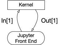
The code cells are numbered and the code within them goes to a kernel (Python 3, in this case) that execute it, and sends it back to the Frontend, which is in charge to display the results in the nicest way possible. A Jupyter session can have many kernels started at the same time, basically one for each open notebook. Take a look at the list of active kernels and shutdown the ones that you don't use. The notebook you are working on will still be opened, and you can continue editing, it is just not connected with any kernel at that time.
To send an input cell to the kernel press Shift+Enter to make it happen. The kernel can run locally in the same computer as the frontend, or remotely. To run it locally, beside Python you also need a number of libraries of code. The instructions on how to do that will follow, but you can start learning about Python rightaway.
Jupyterhub is a server program that can start a jupyter session for each user, on demand. This Jupyterhub run in a server in the supercomputer at TSU, for which you need an username and a password. The link for this service is at: https://hpcc.tsu.edu/jupyter. By accepting to have an account here, you agree that you will be respectful and you will not knowingly try to harm or interfere with the operations of this computer.
Let's get to it!
Here is an example of a code cell:
import numpy as np
import matplotlib.pyplot as pl
#comments ....
This code sets up the stage by getting the required libraries. There is no output from this cell, the kernel will quietly look for these library and bring them into the scope.
**Warning**: The code cells in Jupyter can be executed in any order. This can at times be confusing, as it contradicts the conventional computing paradigm where instructions run sequentially. Executing the cell code below before importing the libraries results in an error because Python will not have knowledge about the function linspace, which is a part of numpy library. If at any time you are lost, you can always restart the kernel manually from the Kernel menu.
You should know that every notebook starts its own kernel, and that kernel continues to live even if you close the notebook. The tab "Running Kernels and Terminals" show the list of all active kernels and allows you to shut down ones that you don't need any more.
Note that markdown allows writing math in a notation derived from LaTeX, like this $\int_0^\infty \frac 1{1+x^2}\; dx = \pi^2/2$ (is this even true?). You can edit the text within a markdown cell by double-clicking it, and render it in the styled form with Shift+Enter. A display-style equation is written by using the double-dollar sign symbol, for example:
$$\frac{d^2u}{dx^2} + \omega^2 u = 0$$
BTW, you might be able to recognize this as the equation that governs the dynamics of a Simple Harmonic Oscillator (SHO). The possibility of writing equations together with the ability of displaying graphics in the same document makes Jupyter and ideal instrument for expressing Computational Physics ideas and concepts. And that should be the case because Jupyter itself was invented by a group of physicists! As you may know, the WWW was invented at CERN, also by physicists.
Let's try to model a simple solution for SHO:
ω = 2.0
x = np.linspace(-5,6,100)
u = np.sin(ω*x)
print(u)
New variables x and u are actually vectors with 100 components. The numpy function sin returns at once a vector where each element is the sine of each element in x. Variable names can have greek (and other Unicode) symbols in them. I obtain the letter $\omega$ by typing $\backslash$omega and pressing Tab.
Now we can plot all (x,u) points and join them with lines, to something that looks like a smooth curve, it is actually made out of (many) straight segments.
pl.plot(x,u);

Do you need to know more about the numpy function linspace? You can google it, of course, but the help is available right here.
?np.linspace
The power of Python stays in part in the abundance of documentation, but also in a very large base of users. If you encounter a problem, chances are that other students had the same difficulty, and solutions might be readily available. All published libraries have details about their functions, and example of usage, as you have seen from the previous example. Python itself is well documented at https://docs.python.org/release/3.9.1/
**Programming Assignment:** Copy this file from the shared folder, paste it into your own home folder and open it, so that you can modify it. Any file in the shared folder is read-only, can be viewed, but cannot be written.
Create a new cell below here with Escape and then b; in there, write code to re-assign the two variables with x = 3 and u = 5 and print the result of this calculation: $x^2 + u^2 - 25$.
By the way, if you don't like a cell, you delete it with Escape and x.
Things to do:
- Explore a nice collection of Jupyter notebooks written on many topics.
- Learn more about Jupyter, IPython and their ecosystem from https://jupyter.org